Euler–Bernoulli Beam Theory - Loading Considerations

Loading Considerations

Applied loads may be represented either through boundary conditions or through the function which represents an external distributed load. Using distributed loading is often favorable for simplicity. Boundary conditions are, however, often used to model loads depending on context; this practice being especially common in vibration analysis.

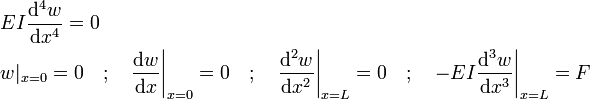
By nature, the distributed load is very often represented in a piecewise manner, since in practice a load isn't typically a continuous function. Point loads can be modeled with help of the Dirac delta function. For example, consider a static uniform cantilever beam of length with an upward point load applied at the free end. Using boundary conditions, this may be modeled in two ways. In the first approach, the applied point load is approximated by a shear force applied at the free end. In that case the governing equation and boundary conditions are:

Alternatively we can represent the point load as a distribution using the Dirac function. In that case the equation and boundary conditions are

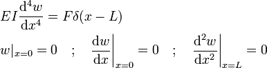
Note that shear force boundary condition (third derivative) is removed, otherwise there would be a contradiction. These are equivalent boundary value problems, and both yield the solution

The application of several point loads at different locations will lead to being a piecewise function. Use of the Dirac function greatly simplifies such situations; otherwise the beam would have to be divided into sections, each with four boundary conditions solved separately. A well organized family of functions called Singularity functions are often used as a shorthand for the Dirac function, its derivative, and its antiderivatives.

Dynamic phenomena can also be modeled using the static beam equation by choosing appropriate forms of the load distribution. As an example, the free vibration of a beam can be accounted for by using the load function:

where is the linear mass density of the beam, not necessarily a constant. With this time-dependent loading, the beam equation will be a partial differential equation:

Another interesting example describes the deflection of a beam rotating with a constant angular frequency of :

This is a centripetal force distribution. Note that in this case, is a function of the displacement (the dependent variable), and the beam equation will be an autonomous ordinary differential equation.